by Neng-Fa Zhou, Brooklyn College, CUNY, USA
Salvador Abreu, University of Evora, Portugal
Ulrich Neumerkel, TU Wien, Austria
PDF Version
The authors participated as a team in the 17th Prolog Programming Contest held with ICLP’2010 in Edinburgh. The contest organizer, Tom Schrijvers, gave our team a special treatment, permitting us to use B-Prolog (the officially supported systems were SWI-Prolog and Yap). We had never been on a team before, so we felt that we needed to practice as a team. Salvador and Neng-Fa got the set of problems used for last year’s contest. No one of the team participated in that contest nor had anyone seen the problems before. There were five problems in the set. As always the set began with a printing question. There were two dynamic programming problems and two constraint problems. The printing problem seemed time-consuming, so we worked on the other four problems. Within a little over one hour, we solved all four problems. Later Ulrich joined and worked out a program for the printing problem.
We made full use of the new features of B-Prolog: loops for printing and constraint generation, mode-directed tabling for dynamic programming problems, and CLP(FD) for constraint problems. The resulting programs are very compact. The top three teams in the 16th contest each solved four problems within two hours (we salute the teams!). How well would have we performed had we participated in that contest? You never know, but we could say that the contest would have been less stressful to our team thanks to the new features of B-Prolog.
In this article we present the programs we wrote during the warm up period. Several minor improvements were made in the midst of writing of this article. All the programs were tested with B-Prolog version 7.4. For each problem, we explain the method and the B-Prolog features used in the solution.
In the real contest, the top two teams including our team each solved two problems within one hour and a half but our team lost to the winning team by two minutes (we submitted four solutions). We choose the problems for the 16th contest rather the ones we solved in the real contest because these problems are simpler and better illustrate the features of B-Prolog.
Salute to the Flag (flag.pl)
The Prolog Programming Contest flag grows bigger with every edition. Here are those for the first, second and third edition:
  _              _                    _
 (_)            (_)                  (_)
<___>          <___>                <___>
 | |_____       | |_____             | |_____
 | |    |       | |     )            | |     )
 | |    |       | |    (_____        | |    (_____
 | |    |       | |    |    |        | |    |     )
 | |~~~~~       | |~~~~|    |        | |~~~~|    (_____
 | |            | |    |    |        | |    |    |    |
                | |    ~~~~~~        | |    ~~~~~|    |
                | |                  | |         |    |
                                     | |         ~~~~~~
                                     | |
Write a general flag/1 predicate that generates the flag for any edition N on the screen by the goal ?-flag(N). Do not add extra spaces to the left!
Program:
flag(N) :-
   format("  _~n (_)~n<___>~n"),
   NR is 2*N+4,
   NC is 5*N+5,
   new_array(A,[NR,NC]),
   p(A,1,5,N),
   foreach(I in 1..NR, (A[I,2] @= '|', A[I,4]@= '|')),
   foreach(I in 1..NR, J in 1..NC,
           [Aij],                 % Aij is local
           (Aij @= A[I,J],
            (var(Aij) -> write(' ') ; write(Aij)),
            (J == NC -> nl ; true ))).

p(A,I,J,1) :- !,
   foreach(C in 0..4, (A[I,J+C]@='_', A[I+4,J+C]@='~')),
   foreach(C in 1..3, A[I+C,J+4]@='|').
p(A,I,J,N) :-
   foreach(C in 0..4, A[I,J+C]@= '_'),
   foreach(C in 0..3, A[I+4,J+C]@= '~'),
   A[I+1,J+5]@=')',
   A[I+2,J+4]@='(',
   A[I+3,J+4]@='|',
   A[I+4,J+4]@='|',
   A[I+5,J+4]@='|',
   A[I+6,J+4]@='~',
   In is I + 2, Jn is J + 5,
   Nn is N - 1,
   p(A,In,Jn,Nn).
Explanation:
The call new_array(A,[NR,NC]) creates a two dimensional array of dimension NR by NC, where NR indicates the number of rows and NC the number of columns. When an array is created, all the elements are initialized to be different variables. In B-Prolog, a term like A[I,J] is interpreted as an array access if it occurs in an arithmetic expression, in an arithmetic constraint, and as an argument of a call to ‘@=’/2. For example, the call A[I,4] @= ‘|’ unifies the element of the array at <I,4> with the atom ‘|’.
The foreach loop construct is very useful for describing loops. In general, a foreach call takes the following form:
foreach(E1 in D1, …, En in Dn, LocalVars, Goal)
where each “Ei in Di” is an iterator, LocalVars (optional) specifies a list of variables in Goal that are local to each iteration, and Goal is a callable term. The foreach call means that for each combination of values E1 ε D1, …, En ε Dn, the instance Goal is executed after local variables are renamed.
This problem is a good example of recursive graphics. The predicate p(A,I,J,N) fills into the array at <I,J> the shape (a) shown below when N is 1 and the shape (b) when N is greater than 1.
              _____          _____
                  |              )
                  |              (
                  |              |
              ~~~~~          ~~~~|
                                 |
               (a)            (b)
The last call in flags/1 prints out the shape stored in the array. The variable Aij is declared local in the loop.
Splitting a Train (split.pl)
One large train arrives at the shunting yard, and it needs to be split into two smaller trains. Trains consist
of wagons, and each (type of) wagon has an identifier (something ground in Prolog). The three trains – the large one and the two smaller ones – are specified as a sequence of such identifiers (in Prolog, these will be lists of the identifiers). We are lucky: the large train has all the wagons to make the smaller trains, and in the correct order. So it is only a matter of deciding for each wagon to which track it goes, and we are done. This involves changing the track setting and decoupling (for the large train) and coupling (for the smaller trains), and since this takes a lot of time, we want to minimize that. Just one example: suppose there are five types of
wagons (i, c, l, f, and p), the large train is represented by [i,i,c,l,c,f,p,p] and the two smaller trains are [i,c,l,p] and [i,c,f,p] respectively, then it is easy to split the larger one into the two smaller ones by a split represented as [1,2,1,1,2,2,1,2] which means that the first wagon i goes to the first smaller train, the second wagon i goes to the second smaller train, the third wagon c goes to the first smaller train etc. But another split is [1,2,1,1,2,2,2,1] which has one less track change (+ the (de)coupling) so it is a better split.
Write a split/4 predicate whose queries look like
?- split(Large,Small1,Small2,How).
where Large represents a large train, Small1 and Small2 represent the smaller trains, and How is free. The predicate must unify How with a best split.
Program:
split(L,S1,S2,H) :- split(L,S1,S2,0,H,_).

:- table split(+,+,+,+,-,min).
split([],[],[],_,[],0).
split([X|Xs],[X|S1],S2,PrevT,[1|How],Cs) :-
    split(Xs,S1,S2,1,How,Cs1),
    (PrevT == 1 -> Cs = Cs1 ; Cs is Cs1 + 1).
split([X|Xs],S1,[X|S2],PrevT,[2|How],Cs) :-
    split(Xs,S1,S2,2,How,Cs1),
    (PrevT == 2 -> Cs = Cs1 ; Cs is Cs1 + 1).
Explanation:
This is a dynamic programming problem. For each wagon, we add it into either the first smaller train or the second smaller train. The call split(L,S1,S2,PrevT,H,Cs) binds H to a list that tells how the list L is split into two smaller lists S1 and S2, where PrevT indicates the train for the previous wagon (0 in the beginning) and Cs is the number of train changes.
Tabling is used in the solution. In a traditional tabling system, all the arguments of a tabled call are used in variant checking and all answers are tabled for a tabled predicate. Mode-directed tabling amounts to using table modes to control what arguments are used in variant checking of calls and how answers are tabled. In general, a table mode declaration takes the form
:-table p(M1,…,Mn):C.
where p/n is a predicate symbol, C (called a cardinality limit) is an integer which limits the number of answers to be tabled, and each Mi (i=1,…,n) is a mode, which can be min, max, + (input), or – (output). An argument with the mode min or max is assumed to be output. The system uses only input arguments in variant checking, disregarding all output arguments. After an answer is produced, the system tables it unconditionally if the cardinality limit is not reached yet. When the cardinality limit has been reached, however, the system tables the answer only if it is better than some existing answer in terms of the argument with the min or max mode (only one argument can be optimized).
The table mode split(+,+,+,+,-,min) instructs the system to table only the answer with the minimum number train changes for each given tuple of input arguments (the default cardinality limit is one). We can also understand mode-directed tabling model-theoretically. We can imagine that split/6 is a big relation indexed on the input arguments that contains all the true facts of split/6 in the Herbrand base. In this example, the relation is finite but in general such a relation can be infinite. For each call to split/6 with a given tuple of input arguments, only the answer with the minimum number of switches is selected.
Panoz (panoz.pl)
Manhattan has several outlets of the famous Belgian bakery Panoz. During an experiment with a new kind
of chocolate pastry, the old bakery has exploded. A new bakery will be built, somewhere in Manhattan, and this occasion is used to optimize the distribution of all the goodies. Clearly Panoz wants the location in Manhattan which minimizes the maximal (Manhattan) distance from the bakery to any outlet.
Write a predicate panoz/2 whose queries look like ?- panoz(Outlets,Sol). where Sol is the location of the new bakery. The outlet coordinates Outlets are given as a list of tuples, e.g. [(0,1),(0,2),(4,0),(4,3)].
Here is a typical query and its answer:
?- panoz([(0,1),(0,2),(4,0),(4,3)],Sol).
Sol = (2,2)
Of course, Sol = (2,1) would also have been a good solution.
Program:
panoz(Ps, Sol) :-
   Xs @= [X : (X,_) in Ps],
   Ys @= [Y : (_,Y) in Ps],
   X :: min(Xs)..max(Xs),
   Y :: min(Ys)..max(Ys),
   Sol = (X,Y),
   Ds @= [max(X1-X,X-X1)+max(Y1-Y,Y-Y1) : (X1,Y1) in Ps],
   minof(labeling([X,Y]), max(Ds)).
Explanation:
Our solution treats the problem as a constraint optimization problem. It uses list comprehensions. The list comprehension
[X : (X,_) in Ps]
retrieves the x-coordinates from the list of xy-coordinates Ps. In general, a list comprehension takes the form:
[T : E1 in D1, …, En in Dn, LocalVars, Goal]
where LocalVars (optional) specifies a list of local variables, Goal (optional) is a callable term. The construct means that for each combination of values E1 ε D1, …, En ε Dn, if the instance of Goal, after the local variables being renamed, is true, then T is added into the list. Syntactically, the first element of a list comprehension takes the special form of “T : (E in D)”. A list of this form is interpreted as a list comprehension if it occurs as an argument of a call to ‘@=’/2 or in an aggregate arithmetic constraint.
Two domain variables, X and Y, are used to indicate the coordinates of the location to be computed. Note that the same variable names are used in the list comprehensions, but this causes no problem because the variables X and Y in the list comprehensions are local.
The third list comprehension (second line from bottom) binds Ds to a list of distances between <X,Y> and the points in Ps. The call minof(labeling([X,Y]), max(Ds)) labels X and Y such that the maximum distance is minimized.
Three on the Circumference (circ.pl)
Given an undirected tree (specified as a list of edge/2 terms), produce a set of three nodes which determine the circumference of the tree. The circumference of a tree is the maximal sum of the distances between three different nodes A,B,C of the tree, that is the sum of the distance from A to B, B to C and C to A – along the edges of the tree of course, where each edge has length 1.
Below are two trees with corresponding queries and answers.

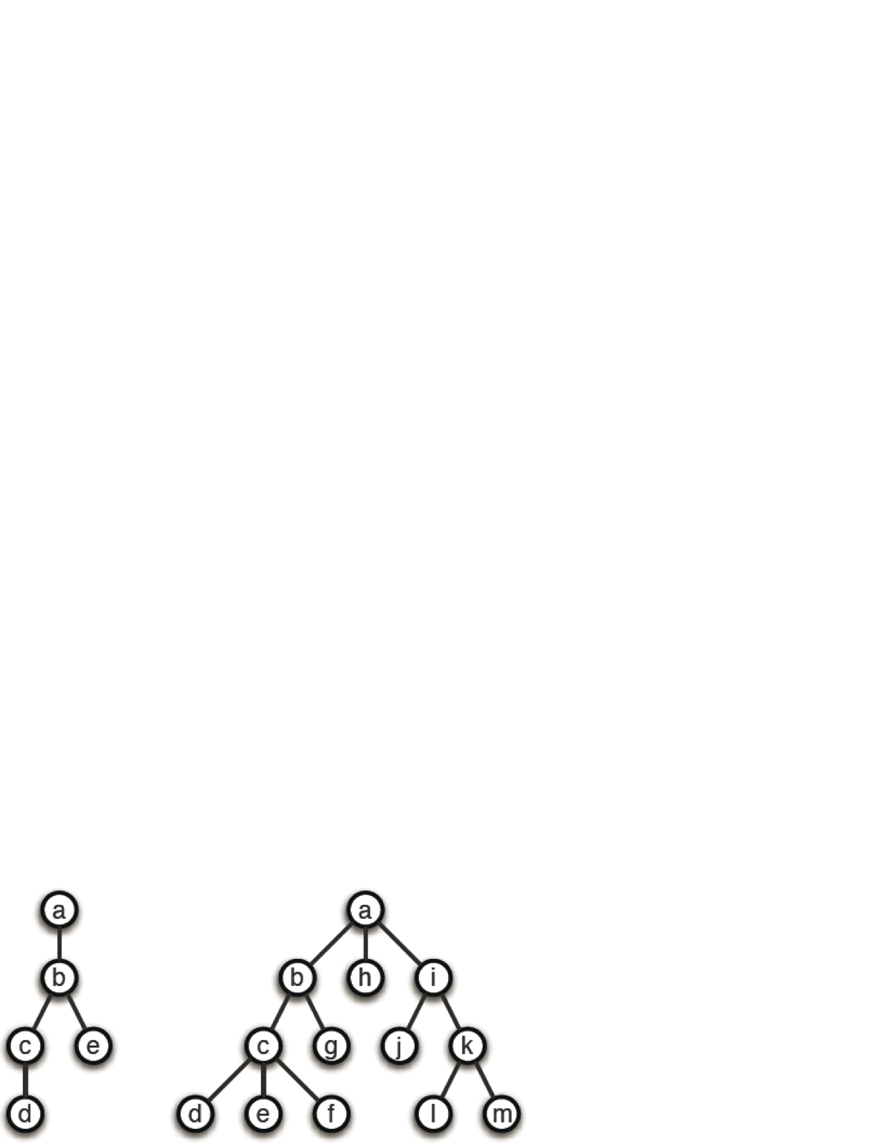
?- circ([edge(a,b), edge(b,c), edge(b,e), edge(c,d)], Three, Len).
Len = 8
Three = [a,d,e]
?- circ([edge(a,b), edge(a,h), edge(a,i), edge(b,c), edge(b,g), edge(i,k), edge(c,d), edge(c,e), edge(c,f), edge(k,l), edge(k,m)], Three, Len).
Len = 14
Three = [d,e,l]
These are of course not the only valid solutions.
Program:
circ(Es, Three, Len) :-
    foreach(edge(A,B) in Es, (assert(arc(A,B)), assert(arc(B,A)))),
    setof(A,B^arc(A,B),Ns),
    L @= [three(Dist,A,B,C) : A in Ns, B in Ns, C in Ns,
                              [Dist],   % Dist is local
                              (A@<B,B@<C,circ(A,B,C,Dist))],
 sort(L, L1),
 last(L1, three(Len,A,B,C)), Three=[A,B,C],
 abolish_all,
 initialize_table.

circ(A, B, C, Dist) :-
 path(A,B,Dab), path(A,C,Dac), path(B,C,Dbc),
 Dist is Dab+Dac+Dbc.

:- table path(+, +, min).
path(A,B,1) :- arc(A,B).
path(A,B,Dist) :-
 arc(A,C),
 path(C,B,Dist1),
 Dist is Dist1+1.
Explanation:
For a given set of edges Es, the foreach call in circ/3 asserts a relation arc/2 into the database. It basically converts the given undirected graph into a directed one. The call setof collects the nodes in the tree as a list into Ns. The list comprehension constructs a list of terms three(Dist,A,B,C) into L by calling circ(A,B,C,Dist) for each triplet of different nodes A, B, and C, where A @< B, B @< C, and Dist is the sum of the distances of the three nodes. The list L is sorted into L1 by the distance and the last triplet in the sorted list is returned as an answer. In the end of circ/3, the call abolish_all removes the asserted relation arc/2 from the database and the call initialize_table cleans up the table area. This post-processing is needed because a program may be queried several times after it is loaded and for a different query a different relation arc needs to be asserted and a different set of answers needs to be tabled.
The predicate path/3 defines the transitive closure of the directed graph. The table mode requires that for each two given nodes only a shortest path is tabled.
Queens, Bishops, and Rooks (bishop.pl)
You know the N-queens problem: put N queens on an N x N board so that no queen attacks any other queen. It is clear that when you have a solution to the N-queens problem, and you replace all queens by rooks, you have a solution to the N-rooks problem. And equally clear is that if you replace all queens in an N-queens solution by bishops, you get a solution to the N-bishops problem. Even better: if in an N-queens solution you replace every queen by either a rook or a bishop, you get a solution to the N-rooks/bishops problem. Indeed, if you replace I queens by bishops and J queens by rooks, you have an (I,J)-solution
(of course, I+J=N). In some (I,J)-solutions, it is possible to add extra bishops, so that no piece attacks any other piece. Obviously, this is never possible in a (0,N)-solution. But in a (3,1)-solution, it is:
 There is even room for one more bishop! For a given N, what is the maximal J so that an (N-J,J)-solution can be extended with at least one extra bishop? Write a predicate bishop/2 which has as input the N and which unifies the second argument with this maximal J. E.g.,
?- bishop(4,N).
N = 2.
Program:
bishop(N, NR) :-
    N>1,
    NR0 is N-1,
    bishop1(2, NR0, NR, N).

bishop1(NB, NR0, NR, N) :-
    bishop(NR0,NB,N), !, NR=NR0.
bishop1(NB, NR0, NR, N) :-
    NR1 is NR0-1,
    NB1 is NB+1,
    bishop1(NB1, NR1, NR, N).

bishop(NR, NB, N) :-
    length(Rs, NR),
    length(Bs, NB),
    Rs :: 0..N*N-1,
    Bs :: 0..N*N-1,
    foreach(I in 1..NR-1, Rs[I] #< Rs[I+1]),   % symmetry breaking
    foreach(I in 1..NB-1, Bs[I] #< Bs[I+1]),
    %
    foreach(I in 1..NR, J in I+1..NR,
            [R1,R2],  % local vars
            (R1@=Rs[I], R2@=Rs[J], rr(R1,R2,N) )),
    foreach(I in 1..NB, J in I+1..NB,
            [B1,B2],  % local vars
            (B1@=Bs[I], B2@=Bs[J], bb(B1,B2,N) )),
    foreach(R in Rs, B in Bs, rb(R,B,N)),
    %
    append(Rs, Bs, Ps),
    labeling_ff(Ps).

rr(R1, R2, N) :-
    R1//N #\= R2//N, R1 mod N #\= R2 mod N.

bb(B1, B2, N) :-
    X1#=B1//N, X2#=B2//N, Y1#=B1 mod N, Y2#=B2 mod N,
    abs(X1-X2) #\= abs(Y1-Y2).

rb(R, B, N) :-
    R//N #\= B//N,
    R mod N #\= B mod N,
    X1#=B//N, X2#=R//N, Y1#=B mod N, Y2#=R mod N,
    abs(X1-X2) #\= abs(Y1-Y2).
Explanation:
For a given size N, we begin trying to find a configuration for N-1 rooks and 2 bishops. If there is no configuration, we decrement the number of rooks by one and increment the number of bishops by one. We continue this until we find a configuration. The number of rooks in the configuration is the number to be returned.
Let NR be the number of rooks and NB the number of bishops. To find a configuration for these pieces, we create a list of NR variables Rs and a list of NB variables Bs. The domain of each variable is from 0 through N*N-1, where N is the size of the board. For each I, the constraints Rs[I] < Rs[I+1] and Bs[I] < Bs[I+1] are generated to break symmetry. Note that in an arithmetic constraint, Rs[I] denotes the Ith element of Rs, counting from 1. For the array access notation A[I], while it takes constant time to access the Ith element if A is a structure, it takes linear time when A is a list. To achieve constant-time access, we should convert lists into structures. Nevertheless, in CLP(FD) programs where constraint solving normally dominates over constraint generation, such an effort may not worth it.
The constraint rr(R1,R2,N) ensures that the two rooks R1 and R2 do not attack each other (the constraint R1//N #\= R2//N ensures that the rows are different and the constraint R1 mod N #\= R2 mod N ensures that the columns are different), the constraint bb(B1,B2,N) ensures that the two bishops B1 and B2 do not attack each other, and the constraint rb(R,B,N) ensures that rook R and bishop B do not attack each other. The foreach construct is used to generate the constraints, and the built-in labeling_ff is used to label the variables using the so called first-fail strategy.
Final Remarks
Like many other languages, Prolog is evolving. New features such as coroutining, attributed variables, constraints, tabling, and loop constructs are being added into Prolog. Unfortunately, a lot of people outside the logic programming community still see Prolog as the old language of three decades ago. The solutions we presented in this article clearly demonstrate the power of some of B-Prolog’s new features: arrays and loops are useful for the printing problem; mode-directed tabling is elegant for the dynamic programming problems; CLP(FD) with loops is powerful for the constraint problems; and list comprehension is useful for constructing lists in two of the programs. It’s hoped that these new useful features will be introduced into other Prolog systems, especially the systems that will be officially supported for future Prolog programming contests. The Prolog programming contest is a very nice thing to have, but to demonstrate the power and beauty of the Prolog language, we also have to go beyond the community. For example, we could form Prolog teams to compete in the functional programming contest and we also could persuade the ACM programming contest to allow Prolog to participate.
Acknowledgement
The set of problems for the programming contest, available at
http://people.cs.kuleuven.be/~tom.schrijvers/PPC16/probs.pdf
was made by Bart Demoen and Tom Schrijvers. Thanks to Tom Schrijvers for testing the solutions and giving us feedback.